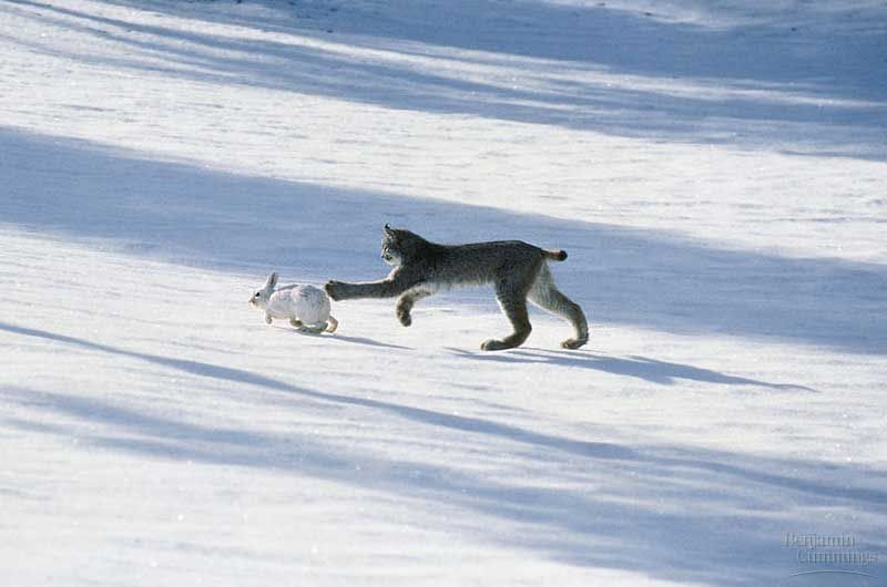
The population of a species that could be observed at a given time with respect to other species in its habitat is an important area of study in ecological mathematics. The availability and competition among species for food give rise to threats and opportunities. This leads to a natural hierarchy of predators and prey. A simple discussion among friends ignited the spark of this topic.

In the mid-1920’s Italian marine biologist Umberto D’Ancona noticed that the average percentage of predatory fish caught in the nets of a port annually fluctuated over time as shown.

This fluctuation grabbed D’Ancona’s interest as he tried to reason out a biological explanation for this. He argued that the population of predatory fish saw a rise in its numbers as fishing activities greatly reduced during the war (1914-1918). This caused an abundance of prey fish and more opportunities for predators. The loopholes in this were the lack of explanation of how fishing would affect the numbers mathematically, and why the lack of fishing did not give rise to the numbers of all fish in the sea. With this in mind, D’Ancona turned to his friend, mathematician Vito Volterra with this issue.

Preliminary Assumptions

Volterra began work on developing a mathematical model of the above scenario using a few constraints and assumptions. The population of a certain species of prey fish at a given time is represented by x_(t). The population of a certain predatory species of the prey at that time is represented by y_(t).

Assume that within a fixed boundary only the populations of the two species above and food (plankton) for the prey fish exist. Further consider that the only threat for the prey fish is the predators present. If there is abundant food for the prey fish, they would not need to compete with each other for food. Finally, assume that immigration and emigration of all species across the boundary are prohibited.

Volterra’s Equation for a Prey Species

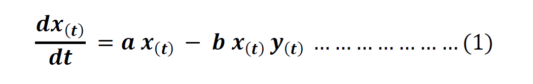
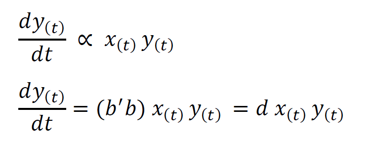
As we saw earlier, without competition factors the prey fish population would grow according to the Malthusian law as follows. Consider that the growth rate, which is the difference between the birth rate and natural death rate of the prey population to be given by the positive constant a.

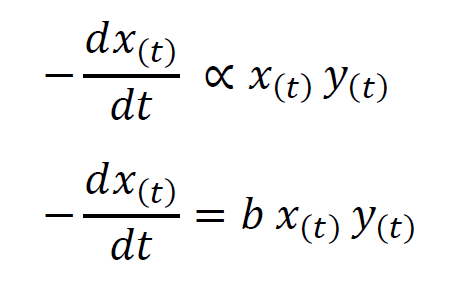
But as data shows the prey population doesn’t grow exponentially implying the presence of a controlling factor. Consider the control factor to be the number of encounters where one member of the predator species kills a member of the prey species. Let that factor be represented by the positive constant b. The number of encounters is proportional to both the population of prey fish at a given time as well as the population of predator fish at that time. Since these encounters give a decrease in the population of prey fish we can represent it as follows.

From these two expressions, we arrive at Volterra’s equation for a prey species.

Volterra’s Equation for a Predator Species

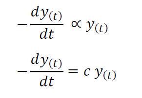
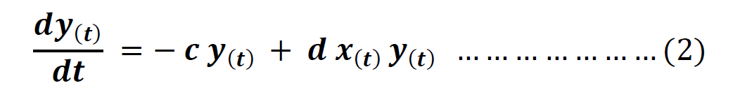
Volterra reasoned that in the absence of the growth in numbers of prey fish, the predatory fish population will decrease proportionally to the population at a given time. Considering the mortality of the predator species to be given by the positive constant c we can represent this as follows.

However, in the presence of prey, the predator population increases with the birth rate of predators. This can be given to be proportional to the number of encounters where a member of the predator species succeeds in killing a prey (b) as well as to the ability of the predators to convert ingested food into offspring (say b’).

From these two equations, we arrive at Volterra’s equation for a predator species.

Analysis of Lotka-Volterra Equations

These equations were similar to those derived by American mathematician Alfred Lotka in 1910 to describe the rates of autocatalytic chemical reactions. Hence the two equations are referred to as the Lotka-Volterra equations or in simpler terms, the predator-prey equations.  Further analyzing this system we can see that it has two stable points as computed below.

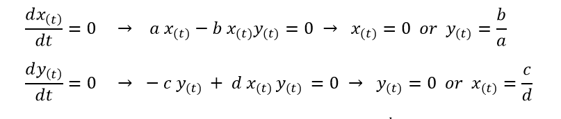
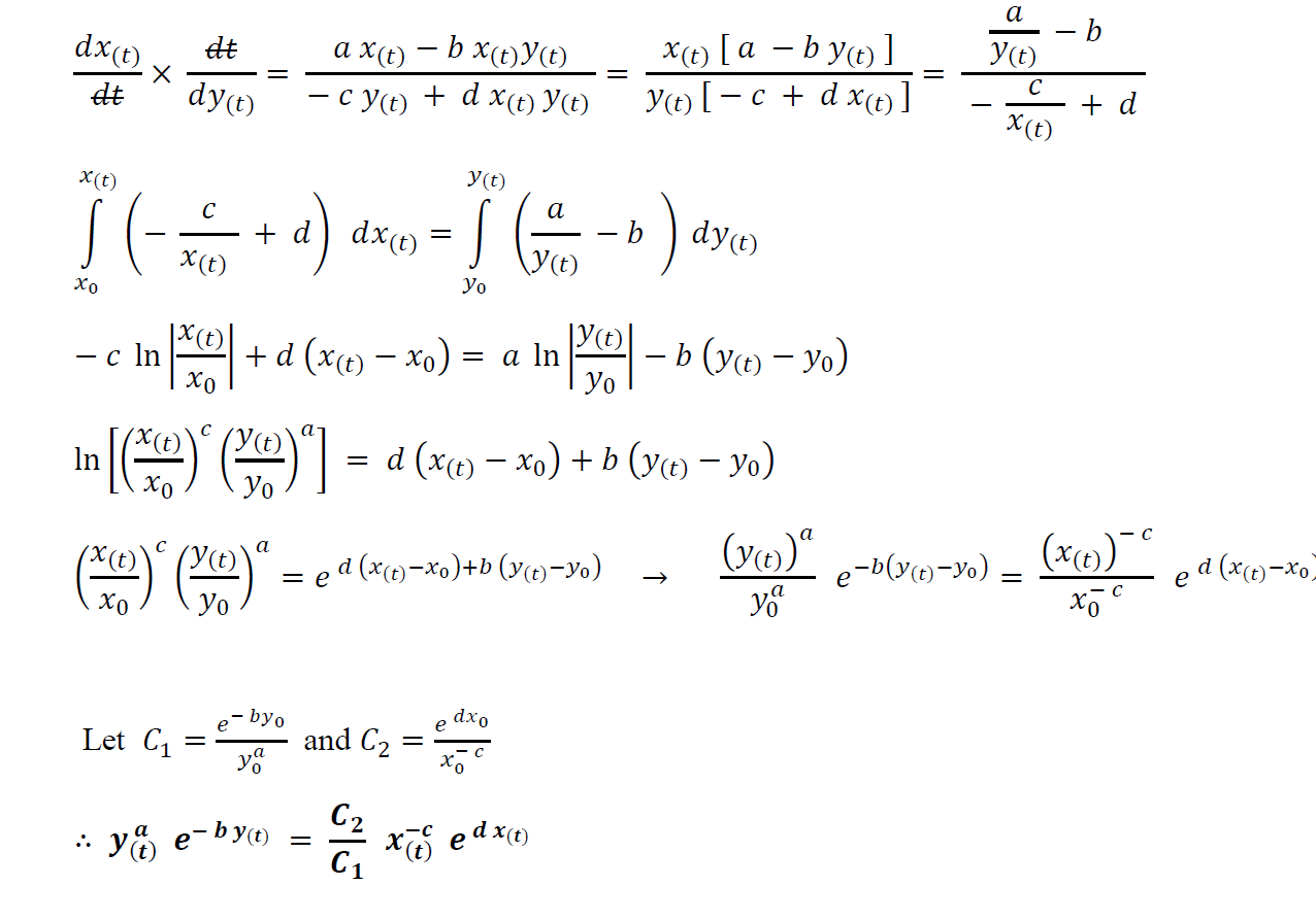
This gives us the two stable points as  (0,0) and (b/a, c/d). First we shall analyze the two equations with respect to each other instead of time. Consider the initial population of prey species as  x₀ and that of the predator species as  y₀.

Dividing (1) by (2):

Graphical Analysis and Inferences

We can represent this solution graphically as follows for the parameters a = 8.8, b = 2.3, c = 4.1, d = 1.1 and  C₁/C₂ = 0.3. Here the horizontal axis represents the population of prey species of fish at a given time (x_(t)) and the vertical axis represents the population of predator species of fish at the same time (y_(t)).

We can identify four stages in this cyclic, oscillatory variation in the populations of the two species as indicated. At Stage 1 the number of predators and prey is small. Since food is abundant for the prey, the prey population will grow at a very high rate eventually reaching a maximum. Meanwhile the predator population grows at a considerably slower rate. At Stage 2 the opportunities for the predators to hunt are at a maximum. Due to this, the predator population will increase until it reaches a natural equilibrium. Here the reproduction rates of both species are at a relatively comparable rate as shown in Stage 3.

With the increase in predator species and the adaptation to using new hunting strategies, the population of predators will rise greatly. Simultaneously, the prey population will decrease until the predator population reaches a saturation point as shown by Stage 4. After this, the high level of competition due to shortages of prey and the law of survival of the fittest applies. This causes a rapid decline in the number of predators as resources thin out. Finally, it cycles back to the initial point of Stage 1.

Graphical Representation of Species Populations

Predator-prey species of similar reproduction rates such as the rabbit and Iberian lynx show a more pronounced oscillation as opposed to the ant and anteater. The reproduction rate mainly depends on the gestation period and the average births per pregnancy of the species concerned.

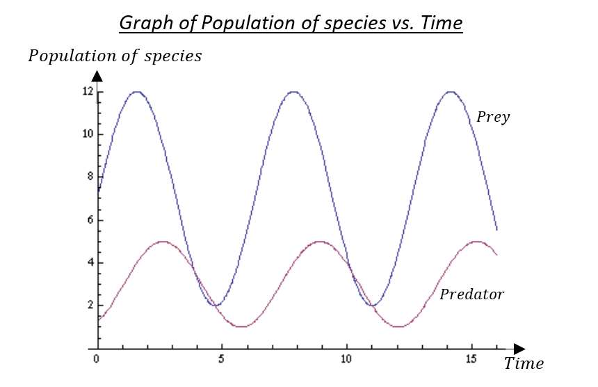
We can see here that the prey population has a higher peak compared to that of the predator population. We can also observe that the predator population lags behind the prey population. The peaks and troughs of each function can vary to different degrees as well with corresponding changes.

Further Insights

Extension of the Lotka-Volterra equations beyond the initial assumptions is possible. By assuming that an abundance of food (plankton) is not available to the prey fish species we can introduce a competition factor into the prey species equation. This model is as described by the Logistics Law of population growth. We can also model linear food chains where the initial predatory species is the prey for another species. Modeling of complex food chains using these equations is also possible. Here we consider a species to be the prey of several predatory species as shown below.

Here we can note that the factor that affects the highest predation level of a species is the success rate of a certain predatory species in killing a prey species member  (b₁ , b₂ , … , b_n). From this, we can take a glimpse into Darwinian evolution. A considerably high evolutionary pressure on a prey species to escape predation through defense mechanisms to reproduce is present. Similarly a pressure on the predatory species to adapt new strategies to oust the other predators to provide food for their offspring present.

An excellent summary of this never-ending swing of near-disastrous extinction to abundance and fertility was given in 1871. To quote the Red Queen from Lewis Carroll’s Through the Looking Glass, “You have to run just to stay in the same place”.

References: 

• Braun, M., 1993. Differential Equations and Their Applications. Fourth ed. New York: Springer Science+Business Media
• Schroeder, J. et al., 2019. The Ecology Book. First ed. London: Dorling Kindersley Limited

Image courtesy: 

• https://bit.ly/3cqUj7O