
“I am telling you, the world’s first trillionaires are going to come from somebody who masters AI and all its derivatives, and applies it in ways we never thought of.”
~Mark Cuban~
Predicting a future is not a dream anymore, cause AI is there with us. Have you ever wondered about how AI has achieved those learning capabilities? It’s not a mission acquired from one night but a huge effort of thousands over decades. Artificial intelligence (AI) is a major branch of computer science that is connected with building smart devices that can perform tasks usually that need human knowledge and intelligence. To make that a deep area of science several concepts and principles have given an irreplaceable impact.
Machine learning (ML) is such an area that defines the necessary algorithms to find and apply patterns in big data through the training and testing process. Machine-learning algorithms use statistics to identify patterns in those big data. And data can come in many forms like numbers, words, images, details. The core of the process of ML is building the models and making the most accurate decisions depending on the interpretations of the model. So ML learns the stuff during the process using statistical regularities or other patterns of data.
Depending on the nature of the learning we categorize ML into several groups like supervised, unsupervised, reinforcement, and semi-supervised learning. In this episode let’s have a deep dive into supervised learning.
- Supervised Learning and the models
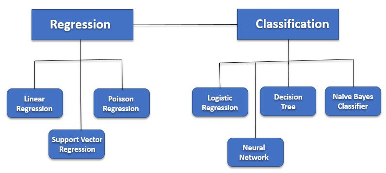
This is defined by its use of labelled data to train the algorithms that to make a decision or classify the outcomes properly. Supervised learning is the most common method for training for neural networks and decision trees as the information based on pre-determined classification is used to learn. Supervised learning is mainly divided into two cases as classification models and regression models.
Let’s take examples for both scenarios. Predicting the prices of a vehicle depending on the features like model, brand, other features of the engine, etc is one of the common examples for regression.
For classification, we can have several example scenarios used in day-to-day life. Classifying spam, Detection by teaching a model of what mail is spam and not spam is the most common application. Speech recognition where we teach a machine to recognize our voice is another well-known example.
Outlining the models, the Regression models take the input for the real-value domain while classifiers map the input space into predefined classes to find out what category they can be put thus very good for practical cases. Apart from that several algorithms go along with supervised learning like the random forest, decision trees, SVMs, neural nets, logistic regression, naive Bayes, memory-based learning, bagged trees, boosted trees, and boosted stumps.
- Linear Regression
Linear regression models the relationship between two variables. For that, it fits a linear equation to observed data. First, we train the model on a set of labeled data (training data) and then use the model to predict labels on unlabeled data (testing data). Here two variables, dependant variable, and explanatory variable are used and the model finds the relationship and dependencies between variables using the linear function. We first plot the graph using the labeled data and acquire the possible line which fits the test set minimizing the value of the loss function.
In this example, we find, how rainfall varies with the year. Thus rainfall is the dependant variable and year is the explanatory variable.

The formula for a simple linear regression is:
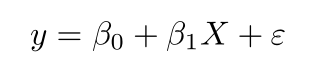
- y – The predicted value of the dependent variable (y) for any given value of the independent variable (x)
- B0 – Intercept, the predicted value of y when the x is 0.
- B1 – Regression coefficient – how much we expect y to change as x increases.
- x – Independent variable
- e – Error of the estimate, or how much variation there is in our estimate of the regression coefficient.
Likewise, after plotting the graph and building the model we then can make predictions on unlabeled data as well.
- Decision trees
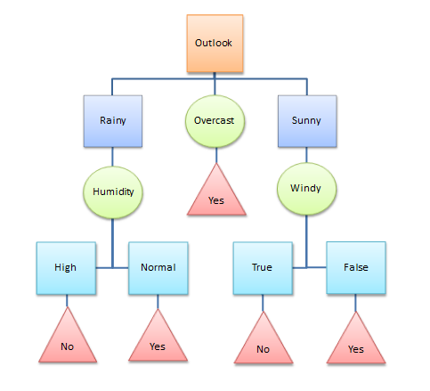
A decision tree is a flowchart-like structure and non-parametric method which consists of nodes and branches. This can be used in both classification and regression problems. Each internal node represents a test on a feature, each leaf node shows the decision taken after computing all the steps. Branches represent conjunctions of features. Those are the vital factors that lead to the decisions. For the practical scenarios, we can apply this most of the time cause it identifies the paths to split the data based on the features or conditions.
To continue with the example of determining the weather of the day has been represented using a decision tree.
- Naive Bayes
It is a classification technique based on Bayes’ Theorem which can be applied even to large data sets making it easy to build the model. It assumes independence among predictors which means that the presence of a particular feature in a class is unrelated to the presence of any other feature. The capturing uncertainly about the model in a principled way is a significant character of this technique.
For example, a vegetable may be considered to be beans if it is green in color, long. Even if these features depend on each other or upon the existence of the other features, we consider that all of these properties independently contribute to the probability of being this vegetable a bean.
Bayes theorem provides a way of calculating posterior probability P(c|x) from P(c), P(x), and P(x|c). See the equation below:
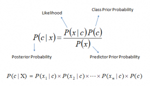
- P(c|x) is the posterior probability of class (c, target) given predictor (x, attributes).
- P(c) is the prior probability of class.
- P(x|c) is the likelihood which is the probability of predictor given class.
- P(x) is the prior probability of predictor.
Anyhow there can be changes in the different naive Bayes classifiers based on the assumptions that they made on the distribution of P(xi∣c).
This is too very famous when comes to document classification and spam filtering as real-world applications. Despite their over-simplified assumptions, these classifiers have worked very well in many scenarios as mentioned earlier. It also performs well in multi-class prediction. Again the decoupling of the class conditional feature distributions means that each distribution can be independently estimated as a one-dimensional distribution which helps to get rid of many issues arising based on the curse of dimensionality. Hence the requirement of the small training data and so fast making it a nicer algorithm to work in ML.
- Logistic Regression
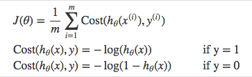
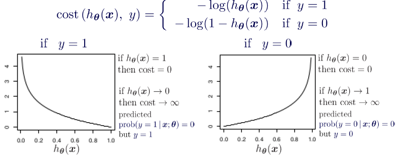
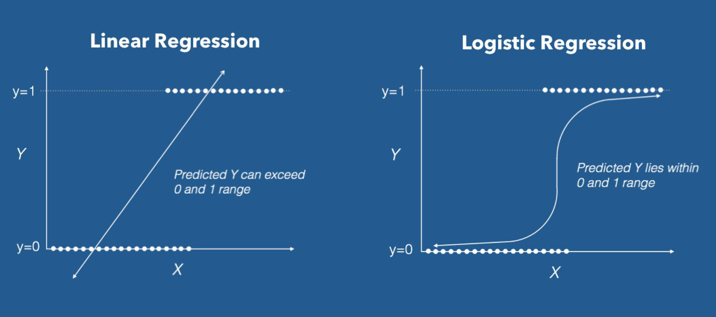
Logistic regression models the probabilities for classification problems with two possible outcomes. This is also known as the logit model. It’s an extension of the linear regression. But uses a more complex cost function (sigmoid, logistic function). The hypothesis of logistic regression usually limits the cost function between 0 and 1. That is why the linear functions fail to represent this model.
This analysis is also mostly used for modeling and also to improve the curtain applications in the ML. The usage of the analysis is to predict the happening of some event or decision. Hence the categorical variable or the finite one can be taken to account. As an example, this can be used in statistical software to understand the relationship between the dependent variable and one or more independent variables. For that, it uses the logistic regression equation in order to estimate probabilities.
For example, predicting cancer for the tumor can be taken. If some particular person is tested for cancer detection, that tumor may be because of cancer or because of any other reason. Based on the analysis we come to the point of either 0 or 1 which signifies diagnosis being positive or negative. But we never try to find any intermediate level in the decision. That is how this analysis works (dependent variable). Therefore logistic regression assumes the dichotomous nature of the dependent variable, assuming that it is binary too; in other words, coded as 0 and +1. It is just like the normal way for 0 to indicate that the event did not occur and for 1 to indicate that the event did occur.
When we pass the inputs through a prediction function classifier identifies the probabilities of data and categorizes them into classes., and returns a probability score between 0 and 1. Therefore we called that the decision boundary is there at the logistic regression.
For Example, We have 2 classes, let’s make them like birds and butterflies(1 — birds, 0 — butterflies). We decide with a threshold value above which we classify values into Class 1 and if the value goes below the threshold then we classify it in Class 2.
When using linear regression we used a formula of the hypothesis.
hΘ(x) = β₀ + β₁X
For logistic regression, we are going to modify it a little bit.
σ(Z) = σ(β₀ + β₁X)
We have expected that our hypothesis will give values between 0 and 1.
Z = β₀ + β₁X
hΘ(x) = sigmoid(Z)
hΘ(x) = 1/(1 + e^-(β₀ + β₁X)
Logistic regression is used in thousands of fields. For examples machine learning, the most medical field for disease detection and scoring, and social sciences to identify behaviors and networks can be identified. The prediction of some diseases is a nice example of this and (TRISS) the Trauma and Injury Severity Score is the method developed using the logistic regression. Again in the marketing strategies in social media can be improved using this analysis paying our attention to the possible audience and visitors and their usage frequency of certain pages or a site in order to make them better versions in the marketing strategies.
Apart from those theories, there are many applications and concepts in Supervised learning nowadays. Thus, in the past few years, there has been a rapid rise in the use of SL in many fields like risk assessment in financial services or insurance domains, image classification like Facebook recognizes our friend in a picture from an album of tagged photos. , fraud detection to identify whether the transactions made by the user are authentic or not, and visual detection as well.
Thus the SL has achieved many a thousand milestones in its journey. To conclude there is a nice comment which Elon Musk wrote in a comment on Edge.org, “The pace of progress in artificial intelligence is incredibly fast. Unless you have direct exposure to groups like Deepmind, you have no idea how fast it is growing at a pace close to exponential. The risk of something seriously dangerous happening is in the five-year time frame. 10 years at most.” Therefore next decades are too likely to witness a considerable rise in many more applications. Surely, the universe is full of intelligent life. It’s just been too intelligent to come here. Let us welcome new intelligence.
Image Courtesies:
- Featured Image: https://bit.ly/30vZ0g7
- Figure 1: https://bit.ly/3ndRJJF
- Figure 2: http://bitly.ws/hj3P
- Figure 3: http://bitly.ws/hj3Q
- Figure 4: http://bitly.ws/hj4m
- Figure 5: http://bitly.ws/hj3X
- Figure 6:http://bitly.ws/hj3Z
- Figure 7: http://bitly.ws/hj46
References :
- https://towardsdatascience.com/decision-trees-in-machine-learning-641b9c4e8052
- https://www.ibm.com/cloud/learn/machine-learning
- https://gauthamsanthosh.medium.com/understanding-naive-bayes-in-real-world-3c4da612a0cf
- Pattern Recognition and Machine Learning (1st Edition) by Christopher M. Bishop