
In the physical world around us, we often talk about energy as a transferrable quantity. This transfer happens not only from one form to the other but also from one physical body to another. In this study of a back and forth relationship of energy, we come across vibrations frequently. For this, understanding the motion of a single oscillator in undamped and damped scenarios is an important fundamental step. However, we can find that in nature, oscillators rarely exist in complete isolation. In the quest to properly understand the way that energy propagates thus, we come to the discussion of coupled oscillators.
Coupled Oscillations: Preliminary Setup
Here, let’s consider two equal masses each of mass m coupled together by a spring of constant k. Here we can denote the angles the strings make with the vertical measured in an increasing sense as θ1 and θ2 respectively and the extensions by each string as x1 and x2 respectively. This is as shown below.
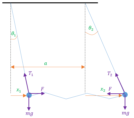
Let’s consider the strings to be of the same length l here. If the initial unstretched length of the spring is a then by applying Hooke’s Law we can write down an expression for the restitution force F acting on the masses as F = k(x2 – x1). Let the mass on the right be labeled as P2 and that on the left be labeled as P1.
Let’s assume here that resistive forces such as damping are not present in this theoretical model and that the oscillations occur in such a way that the maximum angular displacement of the string lies in the small-angle approximation limit for trigonometric identities.
Where the Math Leads To
What follows is a simple procedure of applying Newton’s Second Law to the objects separately and then finding a suitable representation for them.
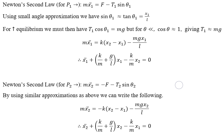
We can get a more meaningful representation for this by assigning new quantities in place of the expressions found above by taking g/l = ω02 and k/m = ωs2.
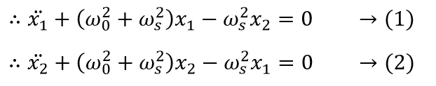

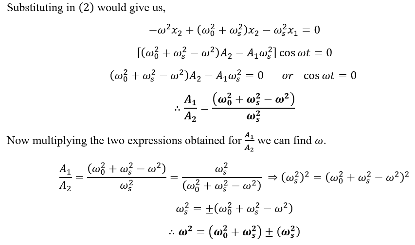 We can see here now that we have two possible values for the quantity ω that would give us two different relationships between the amplitudes of the coupled oscillators.
Pushing In-phase, Pulling Out-phase
The importance of the expression obtained for ω is that it characterizes the motion of the coupled oscillators into two methods based on its value. These “methods” can be described generally by coming up with an expression for the amplitudes we considered earlier as follows.
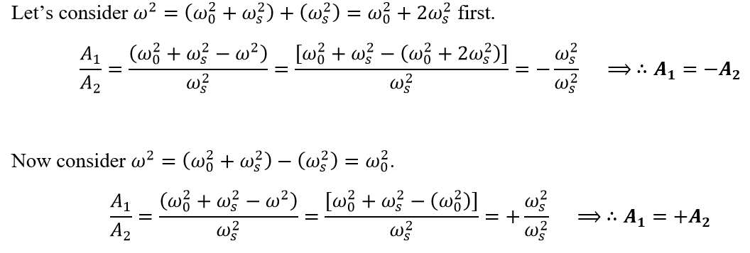
The first case shows that the amplitude of the mass to the right would always be in the opposite direction to that of the mass to the right but of the same magnitude. This can be represented as a Push-Push scenario where if one mass is pushing in one direction, the other mass is pushing in the opposite direction, causing an out of phase oscillation.
The second case however shows a Push-Pull scenario, where if one mass pushes in a direction, the other mass pulls in the same direction. This is termed an in phase oscillation.
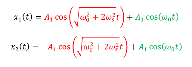
While we can write separate solutions to show these two “methods” in a coupled oscillator, we tend to superpose the solutions for each method together to write the following.
A Constant Push and Pull of Energy
This final expression describing the motions of the two masses gives a very significant result. Here we can see that at one point, the oscillation of mass P1 becomes prominent while that of P2 becomes negligible. And we can see the opposite of this happen at another time interval. However, these two processes occur hand in hand and continue infinitely (theoretically by ignoring resistive effects)!
Furthermore, these “methods” that we found was for a system of 2 particles conducting motion in a 1-dimensional space. In other words, for a system with 2 degrees of freedom, x1 and x2. These methods can then be re-termed as “modes” of energy oscillation.
This is the fundamental step for us to understand how energy propagates in matter and space. However, it is of importance to note that we considered this propagation only as a coupled oscillation between adjacent objects, or in more practical terms, the coupled oscillations between two adjacent molecules. With this understanding, we can now expand this concept to coupled oscillation systems with N number of oscillators present. And in doing so, move from the particulate view obtained here, to the perspective of waves.
References:
01. Pain, H. J. (2005). The Physics of Vibrations and Waves (6th ed.). John Wiley and Sons Ltd., England.
02. French, A. P. (1971). Vibrations and Waves (9th ed.). Massachusetts Institute of Technology Press, United States of America.
Image Courtesies:
01. Featured Image: https://bit.ly/3teBvDC (Customized by Umesha Abeysuriya)
02. Image 01: Author illustration.
03. Image 02 (GIF): https://bit.ly/3tfkKbw